Finally, it’s time for some actual examples of (very very simple) Bayesian analysis. The last part of the chapter gives a summary of “how to do Bayesian analysis,” and Kruschke walks through the skeleton of steps that you need to do in order to use the code and concepts developed up to this point to analyze some (binary categorical) data. If you are working through this book yourself, I highly recommend the exercises. There is a lot of pedagogical value there, so much that I think this chapter would be incomplete if you skipped them. In this post, I will walk through some analyses with some additional data, comparing the Bayesian results to a traditional analysis, and illustrating a few points I find interesting.

Kruschke provides a lot of code, here and throughout the book. However, while these code examples work well to get through the examples and exercises, they are not necessarily well-suited to trying out other things. For example, the BernBeta function in the BernBeta.R script crams a whole lot of stuff into it. In addition to plotting the prior, likelihood, and posterior probabilities, it returns the shape parameters of the posterior. But it prints out some values on the plots (like the HDI information and the value of p(D)) which you can’t access later. So I tweaked the code of this function. I’ll take you through the details in another post. Here, I just want to note that the easiest way to replicate what I show in this post is to clone (or just download) my kruschke_remix repo on GitHub and inspect/run the code yourself, which is contained in a .R script in the “post_code” folder.

The first thing is to load the functions and data we’ll need. Note that I’m trying to keep Kruschke’s original code (which I stole directly from his website) in a separate folder in the repository from the “remix” code, which is first stolen, then tweaked. This is just to help keep track of which code is “original,” and which has been messed with by me.

1
2
3
4
5
6
7
8

source("../code/Chapter5/bernbetaShPsy.R")
source("../kruschke_code/HDIofICDF.R")
std.err.perc <- function(p, n) { sqrt(p*(1-p)/(n)) }

learn <- read.delim("../data/LangLearnPilot.txt")
learn.sub <- droplevels(learn[learn$Apt == "match.CaseB" &
                              learn$Test == 3 &
                              learn$Condition == "CaseB", ])

The lines loading the data are picking out a specific subset of data, just for the sake of illustration, so don’t worry about the details of what the data represents. To simplify things, just assume that this data represents performance on a language test, and that each data point is an independent “correct” or “incorrect” (1 or 0) response, and since there are only two possible responses, guessing should get around 50% correct. And let’s assume that the research question here is whether performance in this task is greater than chance or not. This is analagous to Kruschke’s example of wanting to know whether this is a “fair coin” or not.

One simple traditional way to analyze the data is to compute a standard error for the overall proportion correct, and use a confidence interval of 1.96 times the standard error. That’s what the next couple of lines of code represent (the function for computing the standard error was created in the block above).

1
2
3

mu <- mean(learn.sub$Score)
n <- length(learn.sub$Score)
mu.ci <- c(mu - 1.96 * std.err.perc(mu, n), mu + 1.96 * std.err.perc(mu, n))

The overall accuracy is 41 correct out of 60 (a proportion of 0.683), and the 95% confidence interval goes from 0.566 to 0.801. This basically means we can reject the hypothesis that the “true accuracy” is less than 0.566 or greater than 0.801 (56.6% or 80.1% accuracy), assuming the standard p < .05 level of “significance.” Since we are interested in whether performance was better than chance (better than 0.50), then we can reject the “null” hypothesis that performance was at chance, since a value of 0.50 would be outside the range of 0.566 through 0.801.

So how does a Bayesian analysis differ?

In this chapter, Kruschke has simplified things considerably by picking the mathematical properties of the probability distributions very carefully. Since we are modeling our priors as a beta distribution and the likelihood as the Bernoulli likelihood function, the math works out very nicely, and computing the posterior boils down to just combining the prior and likelihood distributions in a straightforward way. All of this math derives transparently from Bayes’ Rule, and Kruschke goes through it step by step, so I won’t reiterate the details here.

But the basic idea is that we use Bayes’ Rule to compute the posterior distribution, and then find the Highest Density Interval (HDI) corresponding to 95% of the distribution. This has an analagous (though not exactly equivalent) interpretation as a confidence interval, because it’s telling use that the most credible values for the parameter θ (which is the “accuracy” parameter we are curious about) fall within this range. So let’s do the analysis, and see how it stacks up to the traditional confidence interval.

Let’s start with a very simple prior, a shape of (1,1). You can imagine that this is the prior that corresponds to recognizing that there are two possible answers, but you have no idea whatsoever about how responses are expected to pattern. In other words, any value of accuracy is just as expected as any other. So by using this prior, we’re going into the analysis expecting that performance could be 0% accurate, 50% accurate, 100% accurate, or anywhere in between, and all possibilites are equally likely (or unlikely).

The likelihood is a description of how likely the data is (i.e., how likely it is to get exactly 41 correct out of 60) for every possible value of the actual accuracy parameter. So for example, even if you have a coin that is biased to flip heads, there’s still a chance it could flip more tails than heads. Or, if you have a coin that’s perfectly “fair,” the odds are not terribly high that it will flip exactly 50%-50% for any given number of tosses. In terms of our current data, even if the participants have an “at chance” ability to answer the test questions (i.e., they’re just guessing randomly), there’s still a chance they could get 0% correct, 50% correct, 100% correct, or anything in between. So the likelihood says “okay, if we assume θ is 0.50, then the probability of getting 41 out of 60 is such-and-such, if we assume θ is 0.51, then the probability of getting 41 out ot 60 is so-and-so, etc. etc.,” over the whole range of θ values from 0 to 1.

Finally, our posterior tells us, “okay, now that you’ve observed this data of 41 correct out of 60, what should the new distribution of belief about θ (i.e., accuracy) be?” The following code uses my revised version of Kruschke’s BernBeta function to compute the likelihood and posterior, then plots all three: prior, likelihood, and posterior densities, and annotates the plots with some details. This is all mimicking Kruschke’s original code (in a slightly different way). As an added comparison, I’ve plotted our traditional 95% confidence interval with red vertical lines superimposed on the posterior.

1
2
3

bb.post1 <- bern.beta(c(1, 1), learn.sub$Score)
plot(bb.post1)
abline(v = mu.ci, col = "red")

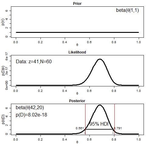
You can see that the values are very similar, though not identical, between the traditional 95% CI and the 95% HDI of the posterior (the red lines representing the CI are very close to the dotted lines representing the HDI). This should be fairly reassuring. And if we think about it, we should probably place a little more faith in the Bayesian HDI, because the CI is based on assumptions about asymptotic behavior, and we really only have 60 observations here. Still, the Bayesian interval is narrower than the CI, so it’s not the case that the CI is less conservative.

But what if we change the prior? Let’s try a prior with a shape of (30, 30). This is similar to saying “we’ve observed 50%-50% behavior from an earlier set of 60 observations” as a prior, which is going to give a preference for belief in accuracy close to 0.50. The following code does this, and gives us some new plots.

1
2
3

bb.post2 <- bern.beta(c(30, 30), learn.sub$Score)
plot(bb.post2)
abline(v = mu.ci, col = "red")

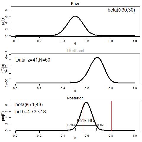
Okay, so let’s stop and notice a few things. First, we see how this new prior differs from the totally flat prior in the previous model, since it is now peaked over 0.50. You can see that values above 0.6 or so, or below 0.4 or so (on the x axis) are pretty low, meaning we have little reason to expect such values. Next, the likelihood is unchanged. This is because it’s still just the probability of the data (for each value of θ), and the data’s still the same. Then note that this change in the prior had a pretty big impact on our posterior! It’s shifted way over, not at all aligned to the traditional 95% CI. But it’s also interesting that the HDI still goes from 0.504 to 0.679. So if all we cared about was whether 0.50 was within the HDI, we’d come to the same overall conclusion, that performance is credibly better than chance.

But notice something else: the actual accuracy we observed was 0.683, and this is just outside the HDI of the second analysis! In other words, given this prior belief we expressed in the second model, we should be pretty surprised to see the pattern of data that we actually collected. This is also captured by the difference in the evidences (remember “evidence” is a technical term that means “probability of data given the model”). This is smaller in the second model (though not that much smaller).

Now let’s try a prior that’s like saying “in a previous set of 60 observations, we saw 2/3rds accuracy.”

1
2
3

bb.post3 <- bern.beta(c(40, 20), learn.sub$Score)
plot(bb.post3)
abline(v = mu.ci, col = "red")

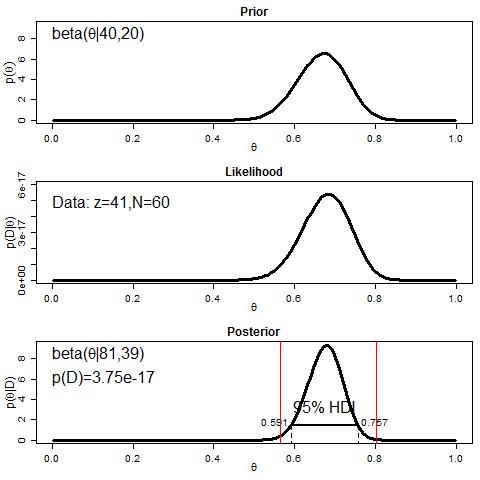
Now you can see that the prior is in a similar place to the likelihood, and the result is a posterior that’s narrower than what we saw in the first analysis. This makes sense because it’s like replicating an earlier set of data pretty closely. That is, the prior is reflecting a belief that we could get by observing 40 out of 60 correct in an earlier experiment, so getting another 41 out of 60 correct is expected to decrease our uncertainty about the exact accuracy level for the test. And decreases in uncertainty mean narrower posteriors, representing a narrower range of credible values. Also notice that now the evidence is more than 10x greater in this model than the previous model (which had a prior peaked over 0.50). Since the priors are the only things that differ between those two models, this is basically saying that this prior peaked over 0.67 or so “fits” the data better than a prior peaked over 0.50.

So now we have two different ways of articulating evidence for the belief that performance in our data is credibly higher than chance (higher that 0.50). First, with a totally flat prior, which gives (perhaps unrealistically) equal likelihood that accuracy on the test could be 0% accurate, 100% accurate, or any value in between, our posterior HDI did not overlap 0.50, meaning that 0.50 is not a particularly believable value for accuracy. Thus we can conclude that performance is greater than chance. Second, we can compare a model that places highest belief in values close to 0.50 (close to chance) to a model that places highest belief around 0.67 (somewhat higher than chance), and see that the second model has a lot more support, given the data. And thus we could argue that since the model with a prior higher than chance is better than a model around chance, it’s more credible that accuracy is above chance.

Is there any difference to taking one of these approaches over the other to make an argument/inference? I’ll be interested to see how these different approaches play out in more involved analyses. But I think in this case, since the choice of a strong prior is fairly arbitrary, it feels simpler to stick with the flat prior (the first model above) and use the HDI to say whether or not performance is above chance (above 0.50). The fact that this lines up closely to a traditional CI derived from the standard error of proportions seems to fit, as well, given the goals of this analysis.

There are several more things I’d like to run through with this simple example, but I’ll save those for some later posts. If any of this discussion raises questions for you, please let me know in the comments!